
Introduction
As a recent transplant from Southern California to the San Francisco Bay Area, one of the differences that immediately stood out to me was the widespread, brazen crime that permeates the area. As someone who analyzes data for a living, I thought it would be interesting to seek out publicly available data on crime to see if I could uncover some truth behind the numbers. The initial intention of this research was to investigate crime rates around the Bay Area to get an idea of some of the trends that have been occurring in recent years, and the main types of crimes that have been occurring. I then thought it would be interesting to leverage additional publicly available data, such as demographic and socioeconomic data, to identify some of the factors associated with higher crime rates in certain towns around the bay, and build a machine learning model to accurately predict crime rates based on various socioeconomic factors.
Data Collection
After conducting some secondary research, I arrived at the 2 primary data sources that were used in this research:
- CA Department of Justice: Crimes and Clearances
- Monthly crime data reported by law enforcement agencies (LEAs) throughout the state of California as part of the FBI’s Uniform Crime Reporting (UCR) program. This information is used to provide statistical data on crimes including criminal homicide, rape, robbery, aggravated assault, burglary, larceny-theft, motor vehicle theft, and arson.
- US Census Bureau:
- DP01 – Decennial Census: Profile of General Population and Housing Characteristics (2020)
- DP02 – Selected Social Characteristics
- DO03 – Selected Economic Characteristics
- S1501 – Educational Attainment
- S1901 – Income in the Past 12 Months (2021 inflation-adjusted dollars)
Crime data was obtained for all LEAs across California (who participate in the UCR program) and US Census data were obtained for the 9 counties and 101 district municipalities that comprise the Bay Area (where available).
Data Cleaning
Quite a bit of cleaning and processing of the data was required before I could dive into the analyses and model development + testing. The detailed process and raw code can be found on my GitHub, but an outline of the methodology can be found below.
I. US Census Data (Demographic, Education, Social, Economic, Income)
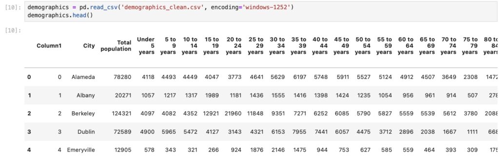
Demographic data (as with all other Census-derived data) was messy and reported in such a way that did not readily allow for analysis. Columns did not represent unique fields, rows did not represent individual entries, numbers were stored as text – it was a mess.
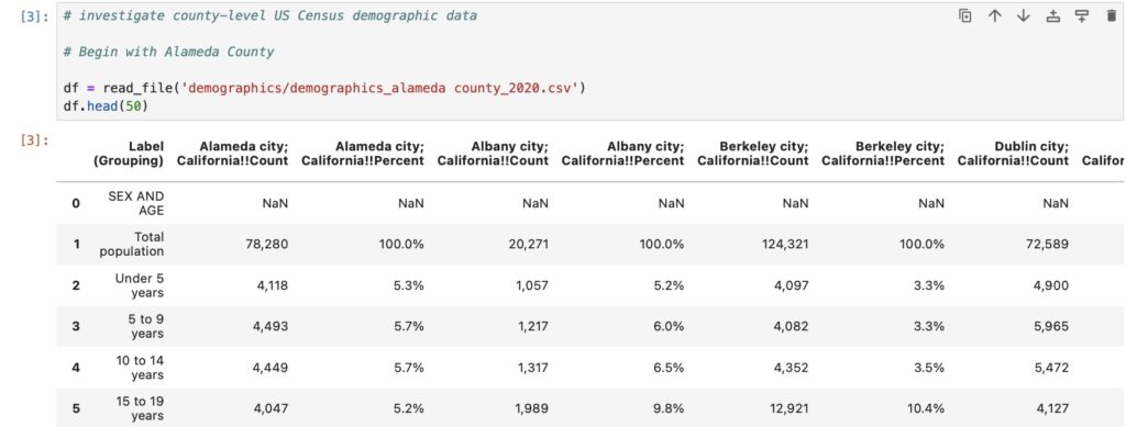
I removed unneeded columns/rows, converted to integer data types and renamed the city/town names accordingly to arrive at a clean, tidy city-level dataset conducive to analysis.
The economic, social, education and income data were reported similarly, thus I followed similar cleaning/reformatting/consolidation steps to arrive at clean, analysis-ready data.
II. Crime Data
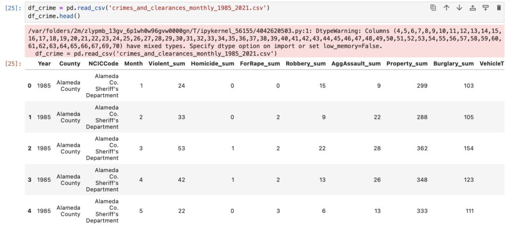
The CA DOJ crime data was reported and delivered in a cleaner format than the Census data, though initial exploration uncovered some necessary cleaning steps that were required before analysis could be conducted (e.g., negative number of crimes in a given month, missing values, etc.). The crime data dates back to 1985 and is reported at a monthly level for all participating LEAs across California, so there were well over 320,000 entries.
Data Exploration
Demographics
Key questions:
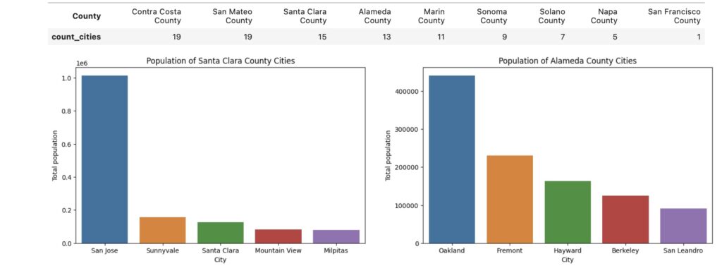
- Which Bay Area cities and counties are the most populous? The least?
- How many individual municipalities comprise the various counties?
- What is the socioeconomic profile of the cities/counties?
- Which cities/counties are the most educated? The least?
- What is the median household annual income across Bay Area cities/counties?
- How do unemployment rates compare between cities and counties?
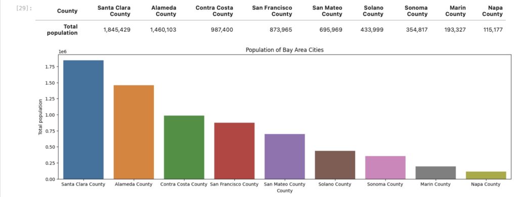
I began by visualizing population rolled up to the county level, noting that Santa Clara and Alameda county lead in total population with over 1 million residents each. Napa and Marin county are at the bottom of the list with less than 200K total residents.
Zooming in on the 2 most populous counties, we see the vast majority of Santa Clara county’s residents are concentrated in San Jose (California’s third largest city by population), with the surrounding towns containing less than 200K residents each. Alameda county’s residents primarily reside in Oakland, though less heavily concentrated than in Santa Clara county.
It is important to note that while San Francisco is 4th in terms of total population, the county is comprised solely of the City of San Francisco, with roughly 900K residents packed onto less than 50 square miles of land surrounded by water.
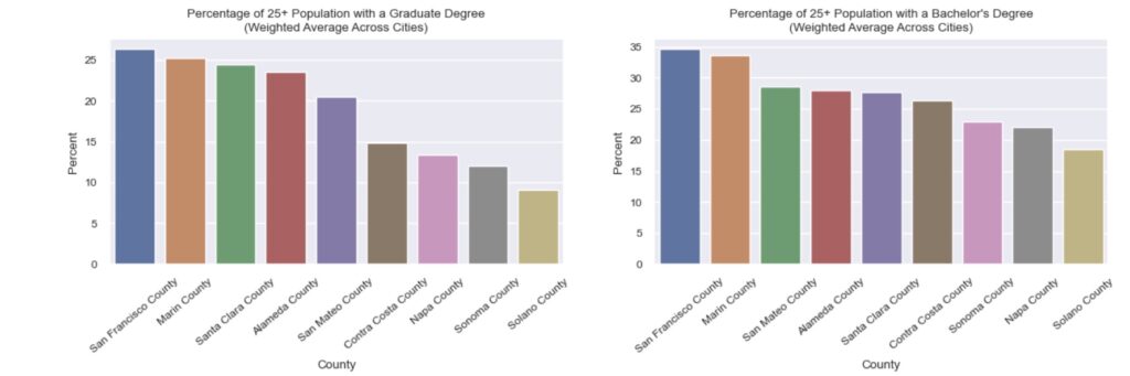
After understanding how the bay area’s population is distributed, I wanted to then understand the socioeconomic profiles of the cities and counties before diving into the crime data. I began by identifying the counties with the most educated and least educated populations aged 25 and above. The proportion of the population aged 25 and above possessing a Bachelor’s Degree, a Graduate Degree, or less than a high school diploma were used to measure the general education level at the city/county level.
San Francisco county leads in terms of overall education level, with >25% of the 25+ population possessing an advanced degree and >1/3rd possessing a Bachelor’s Degree. Solano county is the least educated overall, with the lowest proportion of the population possessing an advanced degree (<10%) or a Bachelor’s degree (<20%), and the highest proportion of the population with only a high school diploma or less.
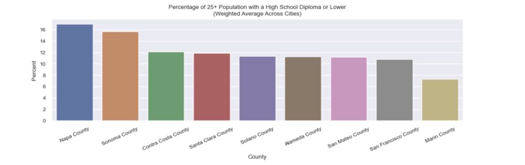
At a city-level, Mountain View (Santa Clara county) and San Anselmo (Marin county) boast the highest proportion of the population with advanced degrees and Bachelor’s degrees, respectively, across the Bay Area. Pittsburg (Contra Costa county) and Hayward (Alameda county) lead in terms of total population with only a high school diploma or less, representing almost half to the population aged 25 and above.
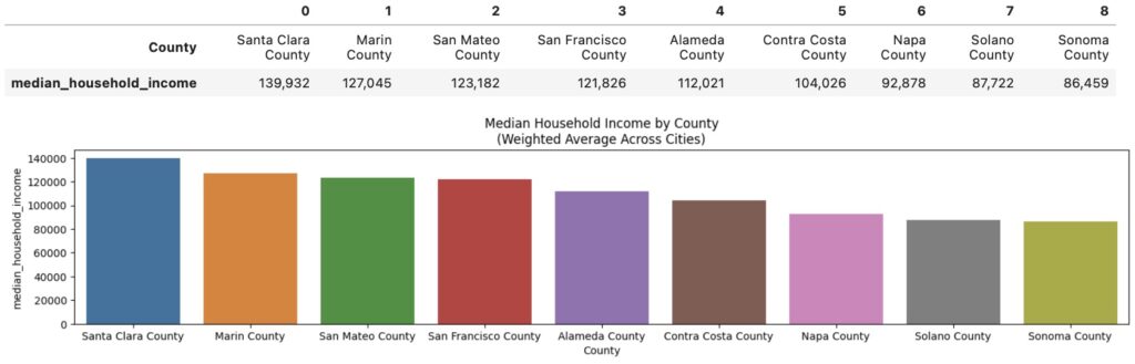
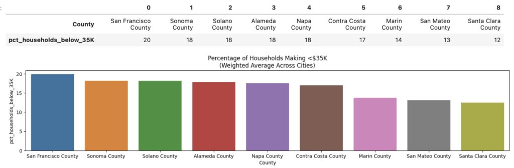
Next, I analyzed economic census data to assess economic profiles across Bay Area cities and counties. From the Census data I calculated unemployment rates, proportion of households making over $150K annually, and proportion of households making $35K or below annually at a city level. There are a number of additional fields that I would be interested in investigating further such as number of workers in specific industries (e.g., construction, manufacturing, education), households receiving supplemental income (e.g., SSI, retirement), and method of transportation to work (e.g., number of workers who drove, walked, took public transit etc.), but limited to few key fields for this research.
Santa Clara county with its 1M+ residents leads in median household income across the Bay Area at $140K annually. With the national median household income at roughly 75K as of 2022, the South Bay Area reflects some of the highest salary opportunities around the nation. Palo Alto holds the top spot with a median household income of almost $200K annually.
Napa, Solano and Sonoma counties fall at the bottom of the list at less than $100K annually.
Unsurprisingly, a similar breakdown is seen when looking at the proportion of households making >$150K annually.
When looking at proportion of low-income households, San Francisco claims the top spot with 20% of households bringing in $35K annually or less, though not by a significant margin.
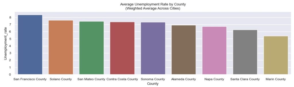
Finally, looking at unemployment rates, San Francisco leads at a county level with over 8% unemployment, followed by Solano and San Mateo counties, though all counties have an average unemployment rate between ~5 and ~8%.
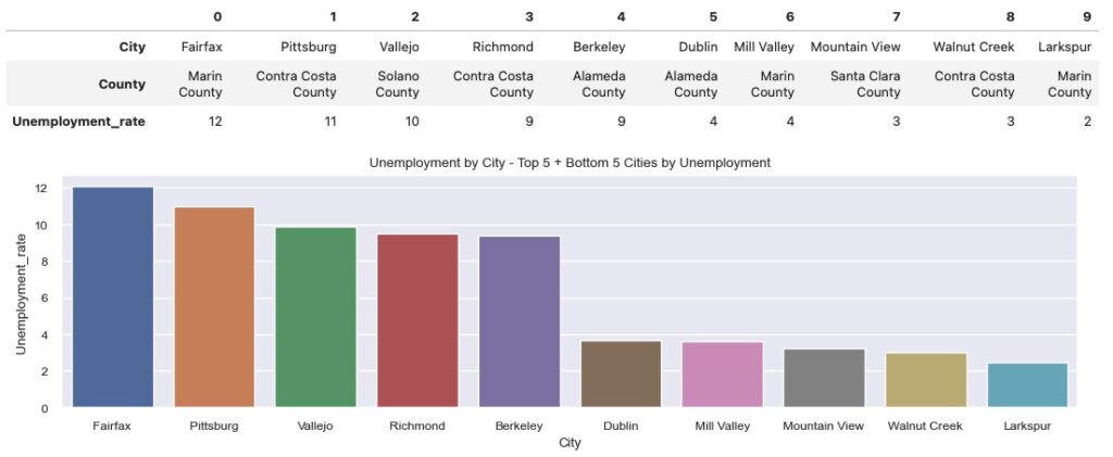
At a city level, Fairfax and Pittsburg lead in unemployment, with 12% and 11% unemployment respectively. Larkspur and Walnut Creek round out the bottom 2 spots, with 2% and 3% unemployment respectively.
Crime
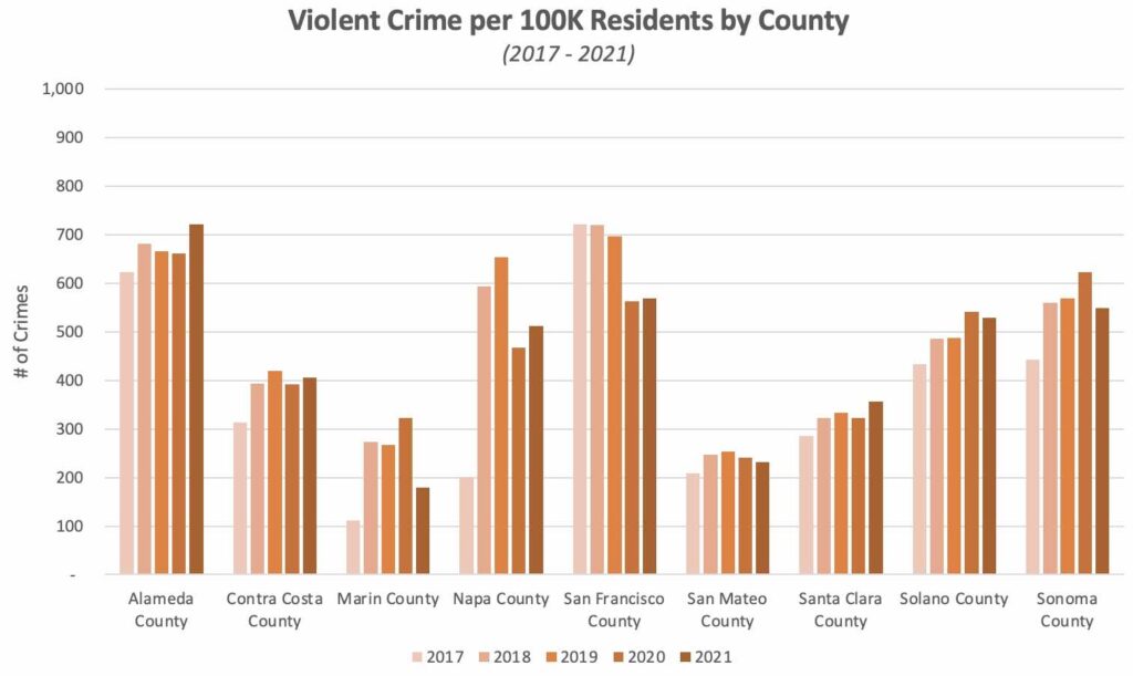
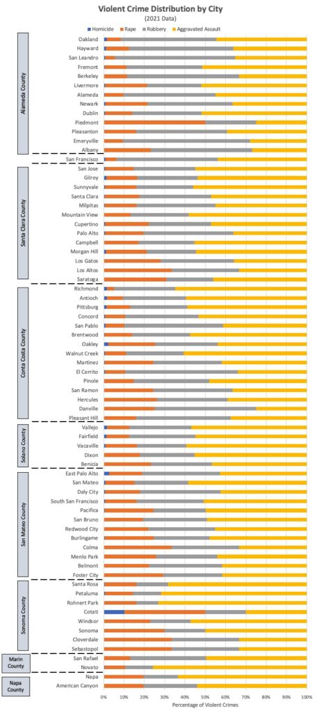
While the crime dataset goes back to 1985, I limited my analysis to 2017 – 2021. The crime data are segmented into 2 key categories: violent crime, which includes homicide, rape, robbery and aggravated assault, and property crime, which includes burglary, vehicular theft, and larceny-theft.
Alameda county leads in overall violent crime per capita, with San Francisco following closely behind. Aggravated assault and robbery are the most common types of violent crime, with Sonoma county and San Francisco county leading in each respective category.
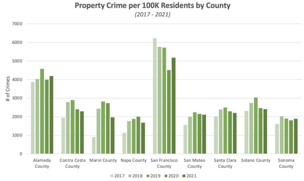
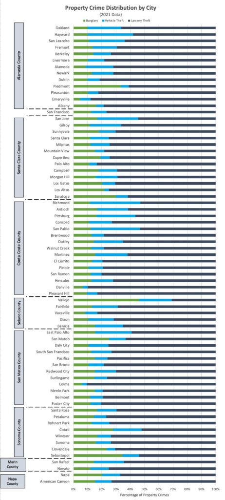
In terms of property crime, San Francisco leads by a wide margin followed by Alameda county. Larceny theft is the predominant type of property crime across the Bay Area, followed by vehicle theft and burglary.
San Francisco County led in violent crime per capita until 2020, when Alameda County jumped to the number 1 spot. Interestingly, while most counties have experienced an overall increase in crime rates over this 5-year period, San Francisco is the only county with a lower per-capita crime rate in 2021 vs 2017.
San Francisco County is the clear leader in property crime per capita across all years, though rates have gradually declined since 2017. While property crime rates are higher across counties in 2021 vs 2017, rates have declines slightly since peak levels in 2019, likely driven in large part by the COVID-19 pandemic.
One dynamic that is not captured here is the exodus of residents out of San Francisco during and after the pandemic, which likely had an outsized impact to San Francisco (estimated ~58,000 people, or 7.2%), with its high cost of living and population density, vs other Bay Area cities.
Model Development
After exploring and cleaning the data, I consolidated the census and crime data to create one master dataset to use for my predictive model. I first mapped correlation rates between the independent variables to note any multicollinearity that may raise issues during linear model development, and arrived at a final list of features to include in the training data for a linear regression model.
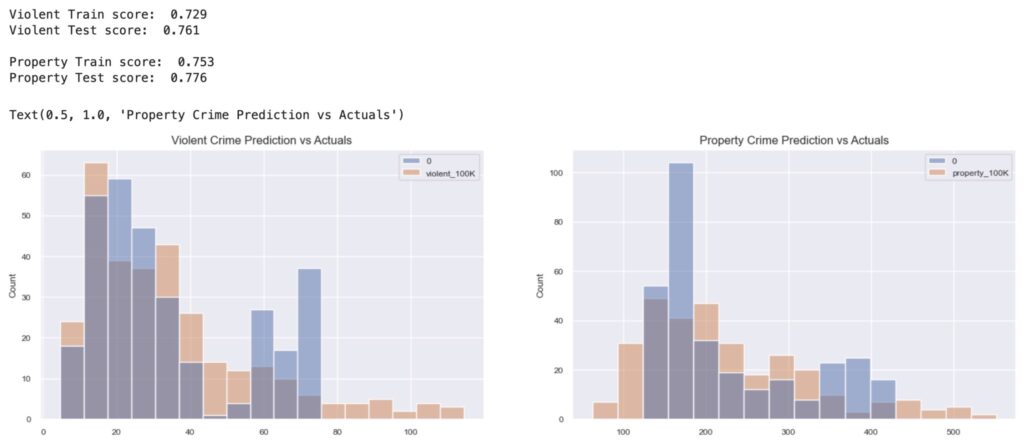
I began by building and training 3 different regression models to predict per-capita violent and property crime rates. I then classified each city as either high crime or not high crime based on per-capita crime being in the 75th percentile among all geographies, and built and trained a Random Forest classifier.
The 3 regression models I tested were a linear model, decision tree, and a random forest ensemble model. While all 3 models scored highly with the testing data, the random forest regression scored the highest, and the liner regression model scored the lowest.
Linear Regression Results
Random Forest Results
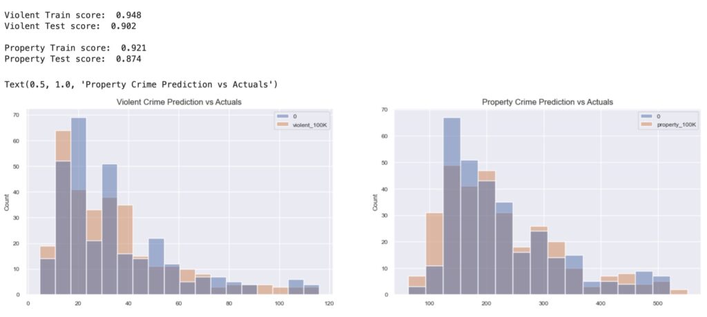
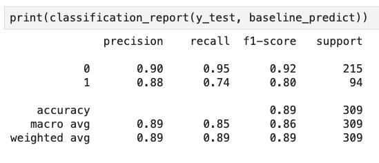
I then created a binary target variable for violent crime and property crime, based on threshold values roughly at the 75th percentile for each target continuous variable. I decided to focus on training a Random Forest classifier and focused on the metrics of precision and recall for predicting ‘high-crime’ geographies. After some hyper parameter tuning I was able to achieve precision of 88% and recall of 74% for predicting a ‘high-crime’ geography.
Random Forest Classification Report
Discussion
Leveraging publicly available monthly crime data across 5 years and socioeconomic data as of 2020, I was able to train a Random Forest classifier to predict a high-crime geography with 88% precision / 74% recall.
Socioeconomic factors such as percentage of working households making less than $35K a year, percentage of the population with advanced degrees (or below a high school diploma), and unemployment rates can be used to predict per-capita violent and property crime rates to a reasonable degree, at least in the San Francisco Bay Area.
As cities and towns across the country have been grappling with increasing crime in recent years, it is important to understand some of the key socioeconomic factors that are associated with, and may be responsible for some of the higher-crime areas such as the San Francisco Bay Area.
There were a few limitations to this research, one being the use of 2020 socioeconomic data across all 5 years of crime data assuming socioeconomic profile remains unchanged during that time. An improved methodology would be to obtain additional city-level socioeconomic data that is reported more frequently, or to extrapolate the estimated population each year based on historical trends. Additionally, given the skewed distribution of the target variables, transformation could have been performed to reduce/remove the skew and potentially increase the accuracy of the linear model.